Building a Fully Reproducible Data Analysis Workflow Using Notebooks and Nextflow

In this post, I will describe a data-analysis workflow I developed to address the challenges I face as a computational biologist:

Ensure full reproducibility down to the exact versions of software used. The irreproducibility of results is a major problem in science. I can tell from own experience that it is really hard to get other people’s code to run, if they did not carefully specify software requirements.
Support mixing of R, Python and Shell commands. Whether R or Python is better often depends on the particular task. Sometimes it’s even preferable to run a command-line tool. Therefore, I want to be able to switch between languages.
Automatic execution on a high performance cluster (HPC). Manually writing job scripts and babysitting running jobs is a pain, the workflow should take care of that automatically.
Automatically only re-execute modified parts. Some steps can be computationally expensive, so it would be nice not having to execute them every time I fix a typo in the final report.
Automatically generate reports and deploy them as a website. A major part of my work is to present the results of my analyses to a non-technical audience (that’s usually Molecular Biologists). This usually involves copying and pasting figures to a word document that is sent around by email – a process that is error-prone and leads to outdated versions floating around.

I achieve this by tying together two well-established technologies: Jupyter and Rmarkdown notebooks on the one hand and the pipelining engine Nextflow on the other hand.

This post in brief

In the following section, I explain why using Jupyter or Rmarkdown notebooks alone is not enough. I will reflect on a few weaknesses of notebooks and propose how to address them.

Next, I’ll introduce reportsrender, a python package I created to facilitate generating HTML reports from both Jupyter and Rmarkdown notebooks.

Finally, I’ll show how to use reportsrender and Nextflow to build a fully reproducible data analysis pipeline.

Reportsrender is available from GitHub. The full example pipeline is available from a separate repository and I suggest to use it as a starting point for your next data analysis project.

Notebooks alone are not enough

Notebooks are widely used among data scientists, and they are a great tool to make analyses accessible. They are an obvious choice to form the basis of my workflow. However, notebooks alone have several shortcomings that we need to address:

Using notebooks alone does not ensure reproducibility of your code. The exact software libraries used must be documented. Moreover, Jupyter notebooks have been critizised for potentially containing hidden states that hamper reproducibility.
Jupyter notebooks don’t allow for fine-grained output control. A feature of Rmarkdown that I’m missing in the Jupyter world is to control for each cell if I want to hide the input, the output or both. This is extremely helpful for generating publication-ready reports. Like that, I don’t have to scare the poor Molecular Biologist who is going to read my report with 20 lines of matplotlib code but can rather show the plot only.
Multi-step analyses require chaining of notebooks. Clearly, in many cases it makes sense to split up the workflow in multiple notebooks, potentially alternating programming languages.
Bookdown and Jupyter book have been developed to this end and allow the integration of multiple Rmarkdown or Jupyter notebooks respectively into a single “book”. I have used bookdown previously and while it made a great report, it was not entirely satisfying: It can’t integrate Jupyter notebooks, there’s no HPC support and caching is “handy but also tricky sometimes”: It supports caching individual code chunks, but it doesn’t support proper cache invalidation based on external file changes. I, therefore, kept re-executing the entire pipeline most of the time.

Fix reproducibility by re-executing notebooks from command-line in a conda environment

In this excellent post, Yihui Xie, the inventor of Rmarkdown, advocates re-executing every notebook from scratch in linear order, responding to Joel Grus’ criticism on notebooks. Indeed, this immediately solves the issue with ‘hidden states’.

We can execute notebooks from command-line through Rscript -e "rmarkdown::render()" or Jupyter nbconvert --execute, respectively. Moreover, we can turn notebooks into parametrized scripts that allow us to specify input and output files from the command line. While this is natively supported by Rmarkdown, there’s the papermill extension for Jupyter notebooks.

If we, additionally, define a conda environment that pins all required software dependencies, we can be fairly sure that the result can later be reproduced by a different person on a different system. Alternatively, we could use a Docker or Singularity container. Nextflow supports either of these technologies out-of-the-box (see below).

Hide outputs in Jupyter notebooks by using a nbconvert preprocessor

While being natively supported by Rmarkdown, we need to find a workaround to control the visibility of inputs/outputs in Jupyter notebooks.

Luckily, nbconvert comes with a TagRemovePreprocessor that allows to filter cells based on their metadata.

By enabling the preprocessor, we can, for instance, add {'tags': ["remove_input"]} to the metadata of an individual cell and hide the input-code in the HTML report.

Use Nextflow to orchestrate multi-step analyses and automate caching

Nextflow is a relatively novel domain specific language designed to build data-driven computational pipelines. It is really easy to get started with and yet very powerful. Wrapping our pipeline in nextflow automatically adresses the remaining issues:

run everywhere: Nextflow abstracts the pipeline logic from the execution layer. Your pipeline will, therefore, run locally, on an HPC or in the cloud with no additonal effort.
caching: Nextflow automatically only re-executes steps that have changed. Based on the input files declared for each process, it properly supports cache invalidaiton.
environments: Nextflow comes with native support for conda, Docker and Singularity. For instance, you can provided a conda yaml file that lists all required dependencies and Nextflow will automatically download them before executing the analysis.

Deploy reports on GitHub pages

By executing the notebooks from the command line, we obtain an HTML report for each analysis step. While you could send them around via email, I recommend to automatically distribute them via GitHub pages. The website serves as a single point of truth and everyone needing to access your results will automatically receive the latest version.

I created the reportsrender package to facilitate building the pipeline

To make these steps as easy as possible, I developed the reportsrender package in Python which wraps Nbconvert and Rmarkdown into a single command. It adds support for hiding inputs/outputs and notebook-parameters to Jupyter notebooks. Both Rmarkdown and Jupyter notebooks are rendered with the same template through pandoc, ensuring consistently looking reports.

Executing and converting a notebook to HTML is as easy as:

reportsrender hello.ipynb hello_report.html

reportsrender hello.Rmd hello_report.html

Through jupytext, reportsrender supports executing arbitrary notebook formats. It can even execute python notebooks with Rmarkdown through the reticulate engine:

# Execute a markdown notebook with nbconvert
reportsrender hello.md hello_report.html

# execute a Jupyter notebook with Rmarkdown
reportsrender --engine=rmd hello.ipynb hello_report.html

Running parametrized notebooks is as easy as

reportsrender hello.Rmd hello_report.html --params="foo=bar"

Using the index subcommand, it allows for generating an index page for github-pages:

reportsrender index --index=index.md first_report.html second_report.html third_report.html

Building the pipeline in nextflow: full example

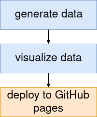
Let’s build a minimal example pipeline that first

generates some data in a Jupyter notebook, then
visualizes the data in an Rmarkdown notebook and finally
deploys the reports to GitHub pages.

The full pipeline including additional recommenations on how to structure the project is available from GitHub.

Here, I will describe step-by-step how to build it.

1. Create a Jupyter notebook that generates the data

Show on GitHub: 01_generate_data.ipynb

Let’s first create a cell that defines the parameters for this notebook (in our case, the output_file).

To this end, define a variable in a cell and add the tag parameters to the cell metadata. This is documented on the papermill website. The declared value serves as default parameter, and will be overwritten if the parameter is specified from the command line.

In [1]: output_file = "results/dataset.tsv"

This parameter can be manipulated from the reportsrender call:

reportsrender 01_generate_data.ipynb 01_generate_data.html --params="output_file=results/data.csv"

Now, let’s generate some data. For the sake of the example, we will just download the iris example dataset and write it to a csv file.

In [2]: import pandas as pd
        iris = pd.read_csv(
            "https://raw.githubusercontent.com/mwaskom/seaborn-data/master/iris.csv"
        )
        iris.to_csv(output_file)

2. Create an Rmarkdown notebook for visualizing the data

Show on GitHub: 02_visualize_data.Rmd

First, we define the input file as a parameter in the Rmd document.

---
title: Visualize Data
params:
   input_file: "results/dataset.tsv"
---

Next, we use ggplot2 to create a plot:

```{r}
library(ggplot2)
library(readr)

iris_dataset = read_csv(params$input_file)

ggplot(iris_dataset, aes(x=sepal_width, y=sepal_length, color=species))
```

3. Create a nextflow pipeline that chains everything together

Show on GitHub: main.nf

The first process takes the Jupyter notebook as an input and generates an HTML report and a csv file containing the dataset. The channel containing the dataset is passed on to the second process. Note that we use the conda directive, to define a conda environment in which the process will e executed.


process generate_data {
    def id = "01_generate_data"
    conda "envs/run_notebook.yml"  //define a conda env for each step...

    input:
        file notebook from Channel.fromPath("analyses/${id}.ipynb")

    output:
        file "iris.csv" into generate_data_csv
        file "${id}.html" into generate_data_html

    """
    reportsrender ${notebook} \
        ${id}.html \
        --params="output_file=iris.csv"
    """
}

The second process takes the Rmarkdown notebook and the csv file as input and generates another HTML report.

process visualize_data {
    def id = "02_visualize_data"
    conda "envs/run_notebook.yml"  //...or use a single env for multiple steps.

    input:
        file notebook from Channel.fromPath("analyses/${id}.Rmd")
        file 'iris.csv' from generate_data_csv

    output:
        file "${id}.html" into visualize_data_html


    """
    reportsrender ${notebook} \
        ${id}.html \
        --params="input_file=iris.csv"
    """
}

The HTML reports are read by a third process and turned into a website ready to be served on GitHub pages. The publishDir directive will copy the final reports into the deploy directory, ready to be pushed to GitHub pages.

process deploy {
    conda "envs/run_notebook.yml"
    publishDir "deploy", mode: "copy"

    input:
        file 'input/*' from Channel.from().mix(
            generate_data_html,
            visualize_data_html
        ).collect()

    output:
        file "*.html"
        file "index.md"

    // need to duplicate input files, because input files are not
    // matched as output files.
    // See https://www.nextflow.io/docs/latest/process.html#output-values
    """
    cp input/*.html .
    reportsrender index *.html --index="index.md" --title="Examples"
    """
}